VeloxQuant-MLX — Fast KV Cache Quantization for Apple Silicon

Algorithms

Eight quantization strategies

Each method targets a different point on the compression–quality–throughput tradeoff curve. New in 0.7.0: RaBitQ 1-bit keys + MSE-b4 values achieves 6× full KV compression on Falcon3-7B — fitting 6× more context in the same memory budget. CommVQ adds RoPE-commutative VQ for exact attention compatibility. Mix and match per layer with RateQuant.

METAL-ACCELERATED IN 0.5.1

VecInfer — Product Vector Quantization

The most aggressive compression method in the library. VecInfer (Yao et al. 2025, arxiv:2510.06175) applies a dual transform to keys before product VQ encoding:

① Smooth scaling — per-channel λ = √(max|K|) suppresses outlier magnitudes
② Walsh-Hadamard rotation — spreads energy uniformly across all dims
③ K-means product VQ — encode sub-vectors against calibrated codebook

The inverse transform is absorbed into queries so q @ K.T is preserved exactly. At 1 bit/elem, a 128-dim key becomes 16 bytes instead of 256 — 16× compression.

New in 0.5.1: hand-written Metal compute kernel for quantize_vq keeps argmin in thread-local registers — 13× faster, 98% less peak memory, no API change required.

Max compression 16× (1-bit)

Metal kernel speedup 6.9× – 14.7×

Peak memory (Falcon3 shape) 729 MB → 12 MB

Qwen2.5-7B throughput 21.5 tok/s vs 21.0 fp16

Calibration required Yes — one-time offline

head_dim constraint Power of 2 only

RVQ

TurboQuant RVQ

Two-pass scalar residual vector quantization. 1-bit sign quantizer + Laplacian residual stage. Achieves 7.5× compression with cosine similarity 0.92, within 5% of fp16 throughput on most 7–8B models. No calibration required.

RATE

RateQuant

Per-layer bit allocation via reverse-waterfilling (arxiv:2605.06675). 1.6s real-activation calibration measures sensitivity per layer and allocates more bits where it matters. Equal quality at lower average bit-width.

POLAR

PolarQuant

Recursive polar coordinate decomposition for clustered key distributions. Lossless angular encoding preserves inner-product structure critical to attention score accuracy.

1-BIT

QJL

Johnson-Lindenstrauss 1-bit sign sketch. An inner-product-preserving random projection for extreme compression scenarios. Minimal memory footprint with provable approximation guarantees.

NEW IN 0.6.0

SpectralQuant — Eigenvector Rotation Quantization

The newest method in the library. SpectralQuant exploits a universal property of transformer KV caches: ~96% of key vector variance concentrates in just 3–4% of dimensions across all architectures. By rotating into the eigenvector basis before quantization, every bit lands on signal — not noise.

① Calibration — one-time SVD over 512 tokens (~5–30s) computes per-layer rotation matrices
② PCA rotation — keys are projected into their principal component basis
③ Signal/noise codebooks — separate quantizers for high-eigenvalue signal dims and low-eigenvalue noise dims
④ No QJL on noise dims — paper finding: QJL correction adds variance without reducing bias on noise dims

New in 0.6.0: calibrate_spectral_rotation(model, tokens) auto-detects architecture (including Gemma 4 multimodal), wraps sliding-window caches, and caches rotations to disk. Works with all mlx-community models.

Compression ratio 5.95× (b=3)

vs TurboQuant 3-bit +7–10pp cosine sim

Qwen2.5-0.5B cosim 0.907 vs TQ 0.833

Gemma 4 4B cosim 0.863 vs TQ 0.758

Calibration time ~5–30s, one-time

Architecture support All mlx-community models

ICML 2025

CommVQ — RoPE-Commutative VQ

Based on Apple ML Research (arXiv:2506.18879). Standard product VQ breaks with RoPE because quantize(rotate(x)) ≠ rotate(quantize(x)). CommVQ trains codebooks on pre-RoPE keys and projects each centroid onto the RoPE-commuting subspace (symmetrising paired dims), so RoPE can be applied exactly at decode time.

Result: 64× key compression (4 uint8 indices for D=128) with exact RoPE compatibility — no attention distortion from positional encoding mismatch.

NEW IN 0.7.0 — FULL KV

RaBitQ — 1-bit Randomised Hadamard Quantization

Based on RaBitQ (SIGMOD 2024) and Ascend-RaBitQ (arXiv:2605.16007). The first method in VeloxQuant-MLX to compress both keys and values, achieving 6× total KV compression on Falcon3-7B.

① IVF clustering — K-Means partitions the key space into nList clusters
② Randomised Hadamard rotation — reuses existing mx.hadamard_transform, O(D log D)
③ 1-bit sign quantization — sign(residual) packed into D/8 uint8 bytes per key
④ Metal Hamming kernel — XOR + popcount scoring via custom rabitq_hamming_score
⑤ MSE-b4 value quantization — scalar TurboQuantMSE at 4 bits for values (4× compression)

Context capacity: at an 8 GB memory budget, fp16 fits ~17k tokens while RaBitQ+MSE fits ~103k tokens — 6× more context in the same RAM. Memory grows linearly with context length at a 6× lower slope.

Key compression (signs only) 11.6× vs fp16

Value compression (MSE-b4) 4× vs fp16

Full KV compression 6× on Falcon3-7B

KV memory @ 1024 tokens 117 MB → 19.7 MB

Context @ 8 GB budget 17k → 103k tokens

Metal kernel rabitq_hamming_score

New in 0.5.1

Hand-written Metal compute kernels

The VecInfer hot path is now a 30-line Metal Shading Language shader, JIT-compiled by mx.fast.metal_kernel on first use. Same Python API; the cache auto-detects Metal and dispatches to the fast path.

Metal kernel benchmark — quantize latency, speedup, and peak memory

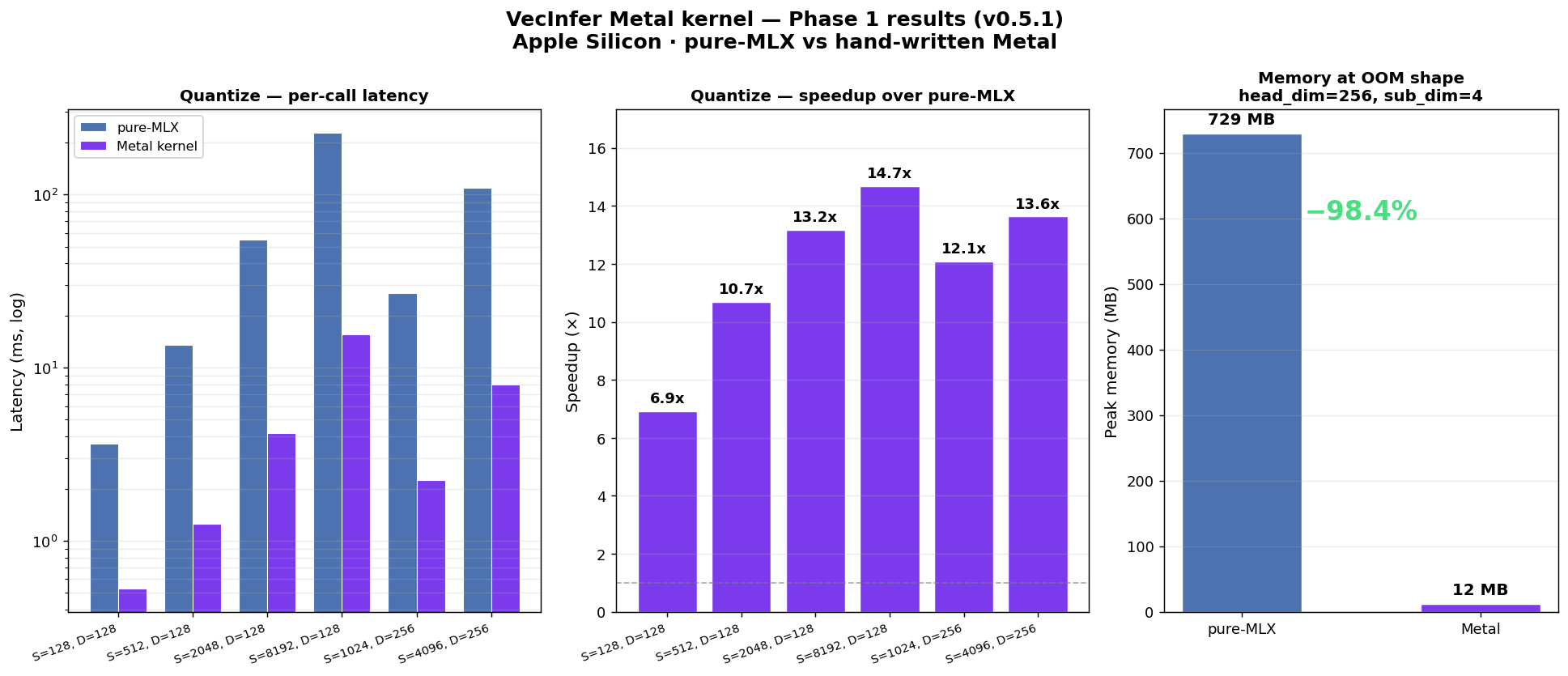
Benchmarked on Apple Silicon GPU.

Quantize latency at S=8192

228 ms → 15.6 ms

14.7× faster per call. The longer your context, the bigger the win — pure-MLX scales linearly with sequence length, the kernel stays flat.

Peak memory at Falcon3-7B shape

729 MB → 12 MB

98% reduction at head_dim=256, sub_dim=4. The argmin accumulator lives in thread-local registers — the [N, n_centroids, sub_dim] diff tensor never gets materialized.

Integration cost

Zero API change

Auto-detected. Opt out with use_metal_kernels=False for parity testing. 7 dedicated parity tests; all 212 tests pass.

Metal Shading Language — the entire fused argmin kernel

// One thread per sub-vector. Argmin lives in registers — no diff tensor.
uint vec_idx = thread_position_in_grid.x;
uint N_total = x_shape[0];
if (vec_idx >= N_total) { return; }

uint n_centroids = codebook_shape[0];
uint sub_dim     = codebook_shape[1];
uint x_base      = vec_idx * sub_dim;

float best_dist = INFINITY;
uint  best_idx  = 0;

for (uint c = 0; c < n_centroids; ++c) {
    uint cb_base = c * sub_dim;
    float dist = 0.0f;
    for (uint i = 0; i < sub_dim; ++i) {
        float d = float(x[x_base + i]) - float(codebook[cb_base + i]);
        dist += d * d;
    }
    if (dist < best_dist) { best_dist = dist; best_idx = c; }
}

out[vec_idx] = best_idx;

Honest caveat: the kernel pays a ~50–200µs launch overhead per call on Apple Silicon. On tiny models (SmolLM2 135M, 30 layers, ~60 launches/token) that overhead can exceed the work saved. The kernel is built for the regime that needs it — 7B+ models with realistic context lengths. Phase 2 (fused dequant + SDPA, never materializing fp16 keys) is on the roadmap. See the full writeup: Metal kernels blog post.

Quickstart

Plug into `mlx_lm` in 3 lines

Same mlx_lm.generate API — just pass a compressed cache.

          python — RVQ 1-bit · 7.5× compression · no calibration
          
        
import mlx_lm
from veloxquant_mlx import KVCacheBuilder, KVCacheConfig

model, tokenizer = mlx_lm.load("mlx-community/Llama-3.1-8B-Instruct-4bit")

# 7.5× key cache compression — within 5% of fp16 throughput
config = KVCacheConfig(method="turboquant_rvq", bit_width_inlier=1, seed=42)
caches = KVCacheBuilder.for_model(model, config)

response = mlx_lm.generate(
    model, tokenizer,
    prompt="Write a 5,000-word analysis of the RLHF literature.",
    max_tokens=5000,
    prompt_cache=caches,
)

          python — VecInfer 1-bit · 16× compression · Metal kernels auto-detected
          
        
import mlx_lm
from veloxquant_mlx import KVCacheConfig, KVCacheFactory
from veloxquant_mlx.allocators.vecinfer import calibrate_smooth_factors, train_codebook

model, tokenizer = mlx_lm.load("mlx-community/Qwen2.5-7B-Instruct-4bit")

# One-time calibration — run once, cache the results
smooth = calibrate_smooth_factors(sample_keys)   # [n_heads, head_dim]
codebook = train_codebook(sample_keys_flat, n_centroids=256, sub_dim=8)

# 16× key compression — Metal kernel auto-detected for 13x faster quantize
config = KVCacheConfig(
    method="vecinfer",
    head_dim=128,
    key_codebook_bits=8,      # 256 centroids
    key_sub_dim=8,             # 16× compression at 1 bit/elem
    smooth_factors=smooth,
    key_codebook=codebook,
    use_metal_kernels=None,      # None=auto, True=require, False=forbid
)
caches = KVCacheFactory.create_for_model(model, config)

response = mlx_lm.generate(
    model, tokenizer,
    prompt="Write a 5,000-word analysis of the RLHF literature.",
    max_tokens=5000,
    prompt_cache=caches,
)

          python — RateQuant · per-layer mixed precision · 1.5-bit average
          
        
from veloxquant_mlx import (
    KVCacheBuilder, KVCacheConfig,
    calibrate_layer_sensitivities,   # 1.6s one-time probe
    allocate_bits_ratequant,          # Theorem 2 reverse-waterfilling
)

# Step 1 — probe real activations
weights = calibrate_layer_sensitivities(model, tokenizer)

# Step 2 — closed-form allocation; average is exact
alloc = allocate_bits_ratequant(weights, target_avg_bits=1.5, beta=3.5)
# alloc = [1, 2, 1, 1, 3, 1, 2, ...]  one int per layer

# Step 3 — build per-layer caches
config = KVCacheConfig(method="turboquant_rvq", bit_width_inlier=alloc)
caches = KVCacheBuilder.for_model(model, config)

          python — SpectralQuant · 5.95× compression · best quality-per-bit · new 0.6.0
          
        
import mlx_lm
from veloxquant_mlx.spectral.calibrate import calibrate_spectral_rotation
from veloxquant_mlx.spectral.spectral_quant import SpectralQuantizer

model, tokenizer = mlx_lm.load("mlx-community/Qwen2.5-7B-Instruct-4bit")

# Step 1 — one-time calibration (~10s). Rotations are cached to disk.
tokens = tokenizer.encode("calibration text here", return_tensors="mlx")
rotations = calibrate_spectral_rotation(
    model, tokens,
    model_name="qwen25_7b",   # cached to ~/.cache/veloxquant/
)

# Step 2 — build per-layer SpectralQuant caches
caches = []
for i, layer in enumerate(model.layers):
    key_U, _, _, _, key_ds, _ = rotations[i]
    sq = SpectralQuantizer(
        d=128, b_signal=3, b_noise=3,
        rotation=key_U, d_s=key_ds, apply_qjl=False,
    )
    caches.append(sq)  # wrap in mlx_lm-compatible cache

# Step 3 — generate as usual; 5.95× compression, +7–10pp quality vs TurboQuant
response = mlx_lm.generate(
    model, tokenizer,
    prompt="Explain quantum entanglement in simple terms.",
    max_tokens=1000,
    prompt_cache=caches,
)

Benchmarks

10 models · 8 configs · Apple Silicon

All numbers from end-to-end mlx_lm.generate with a 200-token prompt, 120-token generation. Apple M-series, unified memory.

Model	FP16 (tok/s)	RVQ-1bit	RVQ compress	VecInfer-1bit	VI compress	Best pick
SmolLM2-135M	250.4	188.5	7.1×	175.8	16×	RVQ-1bit
Llama-3.2-1B	105.4	104.3	7.1×	91.2	16×	RVQ-1bit
Llama-3.2-3B	47.6	46.2	7.5×	40.2	16×	RVQ-1bit
Llama-3.1-8B	20.5	20.6	7.5×	19.6	16×	RVQ-1bit
Mistral-7B	23.6	22.8	7.5×	9.8	16×	RVQ-1bit
Qwen2.5-7B	21.0	20.7	7.5×	21.5 ↑ fp16	16×	VecInfer-1bit
Qwen3-8B	20.3	19.6	7.5×	2.4	16×	RVQ-1bit
Phi-4	10.4	8.1	7.5×	4.0	16×	TQ-2bit (9.6)
Falcon3-7B	17.3	21.7	7.8×	17.0	16×	RVQ-1bit
gemma-3-4b	26.0	24.2	7.8×	22.6	16×	VecInfer-1bit

Highlighted rows — Qwen2.5-7B VecInfer-1bit exceeds fp16 throughput at 16× compression (strong GQA: 28q/4kv heads). gemma-3-4b matches fp16 at 16×. Full per-model plots and raw JSON in figures/vecinfer/ in the repo.

Decision guide

Which method for your use case?

Everyday long-context work

RVQ-1bit

7.5× compression · no calibration · <5% throughput cost on most 7–8B models. The default choice.

Maximum memory savings

VecInfer-1bit

16× compression · one-time codebook calibration · best on models with strong GQA (Qwen2.5, Gemma). Cuts 4 GB cache to 256 MB.

Heterogeneous layer sensitivity

RateQuant

Per-layer allocation · 1.6s calibration · closes the quality gap at fractional average bits. Best on Gemma3, Falcon3 (sensitivity ratio >6×).

Best quality at moderate compression

SpectralQuant

5.95× compression · ~5–30s one-time calibration · +7–10pp cosine sim over TurboQuant. Universal — works on every architecture including Gemma 4 multimodal. Best when quality matters most.

Maximum context length in fixed RAM

RaBitQ + MSE-b4

6× full KV compression · 1-bit keys + 4-bit values · fits 103k tokens in 8 GB vs 17k for fp16 · Metal Hamming kernel · best when context length is the bottleneck.

RoPE-compatible exact VQ

CommVQ

64× key compression · RoPE-commutative codebook (ICML 2025) · exact positional encoding at decode time · no attention score distortion from RoPE mismatch.

Fast KV Cache Quantization
for Apple Silicon

Numbers that matter

Eight quantization strategies

Hand-written Metal compute kernels

Plug into `mlx_lm` in 3 lines

10 models · 8 configs · Apple Silicon

Which method for your use case?

Get started in seconds

Fast KV Cache Quantizationfor Apple Silicon

Numbers that matter

Eight quantization strategies

Hand-written Metal compute kernels

Plug into mlx_lm in 3 lines

10 models · 8 configs · Apple Silicon

Which method for your use case?

Get started in seconds

Fast KV Cache Quantization
for Apple Silicon

Plug into `mlx_lm` in 3 lines