Benchmarking Guide

This guide explains how to use the veloxquant_mlx benchmark CLI, and walks through three real, reproducible worked examples using the scripts in benchmark_scripts/.

CLI benchmark tool

python -m veloxquant_mlx benchmark (veloxquant_mlx/cli/benchmark.py) is a synthetic, model-free microbenchmark: it builds a KV cache directly (no mlx_lm model, no tokenizer) and times cache.attend() against random key/value/query arrays at the sequence lengths you give it. Use it to measure raw encode/attend latency for a given method and bit-width in isolation — for realistic, model-driven throughput/memory/compression numbers, see the worked examples below instead.

PYTHONPATH=. python -m veloxquant_mlx benchmark \
    --method turboquant_prod \
    --bits 2 \
    --seq_lens 512 2048 8192 \
    --compare_optimized

CLI options

Flag	Default	Description
--method	turboquant_prod	One of turboquant_prod, turboquant_mse, qjl, polar
--head_dim	128	Attention head dimension used for the synthetic keys/values
--bits	3	Inlier bit-width
--jl_dim	128	JL projection dimension
--seq_len	1000	Single sequence length to benchmark
--seq_lens	none	Space-separated list of sequence lengths (overrides --seq_len)
--seed	42	Random seed for the synthetic keys/values/query
--compare_optimized	off	Also build a second cache with vectorized attend + fused query-dot + outlier two-stream enabled, and report the speedup vs. the baseline
--n_outlier_channels	4	Outlier channels to protect (only used with --compare_optimized)
--n_calib_tokens	200	Calibration tokens (only used by methods that need them)

Captured output

=== veloxquant_mlx benchmark ===
Method: turboquant_prod, head_dim=128, bits=2, jl_dim=128
seq_len | baseline_attend_ms | optimized_attend_ms | speedup
    512 |             17.103 |               0.794 |  21.536x
   2048 |             48.232 |               0.668 |  72.160x
   8192 |            192.220 |               1.459 | 131.740x

This is attend-only latency on random data, not end-to-end throughput

There's no model, no tokenizer, and no generated text here — keys/values/query are np.random.default_rng arrays, and only cache.attend() is timed. The speedup column compares the same method with and without the optimized code paths (--compare_optimized), not compression vs. fp16. For real end-to-end numbers (tokens/second, peak memory, compression ratio) on an actual model, see the worked examples below — this CLI answers a narrower question: "how much does the optimized attend path help, in isolation, for this method and bit-width."

Worked example: VecInfer

benchmark_scripts/benchmark_vecinfer.py compares three VecInfer configurations (2-bit, 1.5-bit, 1-bit key/value quantization) against a vanilla fp16 KV cache on the same three short prompts, measuring generation throughput, peak memory, and key/value compression ratio for each. It's a good first script to run if you want to see real, reproducible numbers rather than the illustrative snippets above.

PYTHONPATH=. python benchmark_scripts/benchmark_vecinfer.py \
    --model mlx-community/Llama-3.2-1B-Instruct-4bit

The first run performs a short calibration pass (training smooth factors and codebooks on synthetic activations) and caches the result under ~/.cache/veloxquant/vecinfer/<model-id>/, so subsequent runs against the same model are faster.

Captured output

Run against mlx-community/Llama-3.2-1B-Instruct-4bit on Apple Silicon:

Loading mlx-community/Llama-3.2-1B-Instruct-4bit...
  head_dim=64, n_heads=32

--- fp16-baseline ---
  prompt 0: 81 tok in 0.88s (92.1 tok/s)
  prompt 1: 81 tok in 0.70s (115.8 tok/s)
  prompt 2: 81 tok in 0.70s (115.4 tok/s)

--- vecinfer-2bit ---
  prompt 0: 70 tok in 1.00s (70.2 tok/s)
  prompt 1: 78 tok in 0.93s (83.7 tok/s)
  prompt 2: 79 tok in 0.93s (84.8 tok/s)

--- vecinfer-1.5bit ---
  prompt 0: 81 tok in 6.75s (12.0 tok/s)
  prompt 1: 79 tok in 6.68s (11.8 tok/s)
  prompt 2: 76 tok in 6.69s (11.4 tok/s)

--- vecinfer-1bit ---
  prompt 0: 77 tok in 1.20s (64.0 tok/s)
  prompt 1: 82 tok in 1.13s (72.3 tok/s)
  prompt 2: 52 tok in 1.13s (46.1 tok/s)

Summary: figures/vecinfer/Llama-3.2-1B-Instruct-4bit/vecinfer_summary.png
Results: figures/vecinfer/Llama-3.2-1B-Instruct-4bit/results.json

Final:
  fp16-baseline         106.5 tok/s    710.5 MB  key_x=1.00  avg_bits=16.00
  vecinfer-2bit          79.3 tok/s    713.0 MB  key_x=8.00  avg_bits=2.00
  vecinfer-1.5bit        11.7 tok/s    713.6 MB  key_x=10.67  avg_bits=1.50
  vecinfer-1bit          60.9 tok/s    712.9 MB  key_x=16.00  avg_bits=1.00

note

In this particular run, vecinfer-1.5bit was markedly slower (11.7 tok/s) than the 2-bit and 1-bit configs (79.3 and 60.9 tok/s). This is the actual measurement from this script on this machine, not a typo — the 1.5-bit path takes a different, currently less-optimized code path. Re-run yourself before relying on this number; timings are sensitive to thermal state, background load, and MLX/mlx_lm version.

The script saves a 4-panel summary chart alongside a results.json with the same numbers:

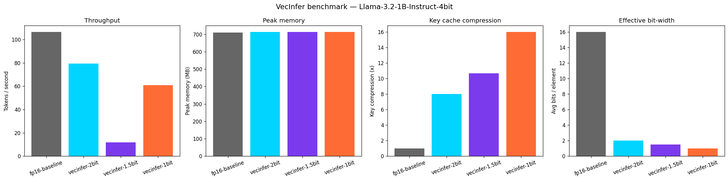
The four panels are, left to right:

• Throughput — tokens/second for each config. Lower-bit configs generally trade throughput for memory savings, though the actual ordering depends on which code paths are optimized (see the 1.5-bit note above).
• Peak memory — peak MLX/Metal memory in MB during generation. In this run all four configs land close together (~710–714 MB) because the model weights dominate total memory at this scale (1B params); the KV-cache savings become more visible at longer sequence lengths or larger models.
• Key cache compression — fp16_key_bytes / compressed_key_bytes for the key cache. This tracks the configured bit-width directly (2-bit ≈ 8×, 1.5-bit ≈ 10.67×, 1-bit ≈ 16×).
• Effective bit-width — the average bits/element actually assigned by the allocator, which should match the config's target (2.0, 1.5, 1.0) — useful as a sanity check that the allocator is behaving as configured.

Try it yourself

Swap --model for any other mlx-community/* checkpoint, and use --max-tokens to change generation length (default 80). Output lands in figures/vecinfer/<model-stem>/ by default, or pass --output-dir to redirect it:

PYTHONPATH=. python benchmark_scripts/benchmark_vecinfer.py \
    --model mlx-community/Llama-3.2-3B-Instruct-4bit \
    --max-tokens 128 \
    --output-dir ./my-results/vecinfer-3b

Worked example: KIVI

benchmark_scripts/benchmark_kivi.py benchmarks several KIVI (arXiv:2402.02750) bit-widths against an fp16 baseline. Unlike VecInfer, KIVI is deterministic — there's no codebook calibration step, so every run is a cold start. KIVI keeps a small fp16 "residual window" of the most recent tokens uncompressed, so the script reports both a key-only compression ratio and a lower full-KV ratio that accounts for that residual.

PYTHONPATH=. python benchmark_scripts/benchmark_kivi.py \
    --model mlx-community/Llama-3.2-3B-Instruct-4bit

Read this before trusting the throughput numbers

This script's own docstring calls out a specific past mistake: an earlier RaBitQ benchmark recorded fp16_ms: 0, which silently invalidated every speedup number derived from it. benchmark_kivi.py was written so the fp16 baseline is always timed for real, specifically to avoid repeating that bug. The docstring also sets an expectation worth stating plainly: on Apple Silicon, KIVI's paper-reported speedup comes from a CUDA kernel that has no Metal port here, so the realistic expectation is a memory win with a throughput cost, not a free speedup. In the captured run below, throughput was actually flat across all configs (~16 tok/s) rather than costly — that's a property of this particular 3B model and short prompt, not a general claim; re-run at longer sequence lengths before drawing conclusions.

Captured output

Run against mlx-community/Llama-3.2-3B-Instruct-4bit on Apple M4 (24 GB):

Loading mlx-community/Llama-3.2-3B-Instruct-4bit...
  head_dim=128, n_kv_heads=8, n_layers=28
  prompt_tokens=2239 (residual_length=32)
  hardware={'platform': 'macOS-26.5.2-arm64-arm-64bit', 'machine': 'arm64', 'chip': 'Apple M4', 'ram_gb': 24.0}

--- fp16-baseline ---
  121 tok in 7.54s (16.1 tok/s)  peak=2484MB  key_x=1.00  fullKV_x=1.00

--- KIVI-2bit ---
  121 tok in 7.39s (16.4 tok/s)  peak=2600MB  key_x=5.79  fullKV_x=3.98

--- KIVI-3bit ---
  121 tok in 7.51s (16.1 tok/s)  peak=2600MB  key_x=4.34  fullKV_x=3.24

--- KIVI-4bit ---
  121 tok in 7.57s (16.0 tok/s)  peak=2600MB  key_x=3.47  fullKV_x=2.73

Results: figures/kivi/Llama-3.2-3B-Instruct-4bit/results.json
  fp16-baseline      16.1 tok/s   2483.7 MB  key_x=1.00  fullKV_x=1.00  toks=121
  KIVI-2bit          16.4 tok/s   2600.1 MB  key_x=5.79  fullKV_x=3.98  toks=121
  KIVI-3bit          16.1 tok/s   2600.1 MB  key_x=4.34  fullKV_x=3.24  toks=121
  KIVI-4bit          16.0 tok/s   2600.1 MB  key_x=3.47  fullKV_x=2.73  toks=121

Peak memory went up, not down, in this run

All three KIVI configs show slightly higher peak memory (2600 MB) than the fp16 baseline (2484 MB) here — the opposite of what compression should do. At this small a model (3B) and short a prompt (~2.2K tokens), the KV cache isn't yet the dominant consumer of memory, so KIVI's bookkeeping overhead (quantized storage + the fp16 residual window) outweighs its savings. Compression wins become visible at longer context lengths, where the KV cache — not the model weights — dominates memory. Try --max-tokens with a much longer prompt to see this shift.

The script saves a 4-panel summary chart alongside a results.json with the same numbers:

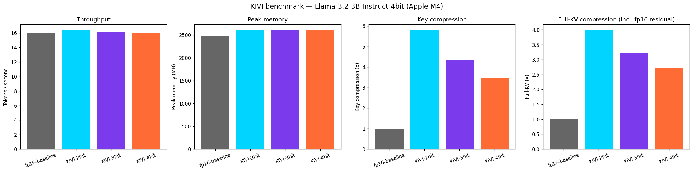
The four panels are, left to right:

• Throughput — tokens/second for each config. In this run all four configs are within noise of each other (~16–16.4 tok/s) — see the caveat above about not over-generalizing from a short prompt on a small model.
• Peak memory — peak MLX/Metal memory in MB during generation. See the note above on why this went up rather than down at this scale.
• Key compression — fp16_key_bytes / compressed_key_bytes for the key cache only. Tracks the configured bit-width (2-bit ≈ 5.8×, 3-bit ≈ 4.3×, 4-bit ≈ 3.5× in this run — lower than the theoretical 8×/5.3×/4× because of quantization group overhead at --group-size 32).
• Full-KV compression (incl. fp16 residual) — the realistic end-to-end ratio once KIVI's fp16 residual window (the most recent --residual-length tokens, kept uncompressed for accuracy) is included. Always lower than key-only compression — this is the number to use when estimating actual memory savings.

Try it yourself

KIVI has more tunable parameters than VecInfer. --model and --max-tokens work the same way; --group-size controls the quantization group size (smaller groups → better fidelity, more overhead) and --residual-length controls how many recent tokens stay in fp16:

PYTHONPATH=. python benchmark_scripts/benchmark_kivi.py \
    --model mlx-community/Llama-3.2-3B-Instruct-4bit \
    --max-tokens 256 \
    --group-size 64 \
    --residual-length 64 \
    --output-dir ./my-results/kivi-3b

Worked example: KVSink protection

benchmark_scripts/benchmark_sink.py benchmarks KIVI-2bit with an added "sink protection" mechanism (method="kivi_sink"): instead of quantizing every token uniformly, a small, configurable number of tokens (k) — typically early "sink" tokens that attention tends to over-weight — are kept in full fp16 precision instead of being compressed. The script sweeps k=0 (plain KIVI-2bit, no protection), k=5, and k=20 against a real-timed fp16 baseline to show the resulting compression-vs-protection tradeoff.

PYTHONPATH=. python benchmark_scripts/benchmark_sink.py \
    --model mlx-community/Llama-3.2-3B-Instruct-4bit

This script does not measure output quality

The script's own docstring is explicit about scope: "without a perplexity harness, quality evidence here is limited to tokens-generated (a coherence proxy); the reconstruction-quality claims are covered by the unit tests on planted-sink data (tests/cache/test_sink_cache.py), not by this script." In other words — this benchmark tells you the throughput/memory/compression cost of sink protection, not whether it actually improves generation quality. If you want evidence that sink protection preserves reconstruction fidelity, look at the unit tests, not this script's output.

Captured output

Run against mlx-community/Llama-3.2-3B-Instruct-4bit on Apple M4 (24 GB):

Loading mlx-community/Llama-3.2-3B-Instruct-4bit...
  head_dim=128 kv_heads=8 layers=28 prompt_tok=2239 hw={'platform': 'macOS-26.5.2-arm64-arm-64bit', 'machine': 'arm64', 'chip': 'Apple M4', 'ram_gb': 24.0}

--- fp16-baseline ---
  121 tok in 7.40s (16.4 tok/s)  peak=2476MB  key_x=1.00  fullKV_x=1.00  sink_fp16=0B

--- KIVI-2bit ---
  121 tok in 7.38s (16.4 tok/s)  peak=2600MB  key_x=5.79  fullKV_x=3.98  sink_fp16=0B

--- KIVI-2bit+sink-k5 ---
  121 tok in 8.79s (13.8 tok/s)  peak=2200MB  key_x=5.80  fullKV_x=3.95  sink_fp16=679936B

--- KIVI-2bit+sink-k20 ---
  121 tok in 8.79s (13.8 tok/s)  peak=2200MB  key_x=5.83  fullKV_x=3.85  sink_fp16=2633728B

Results: figures/kivi_sink/Llama-3.2-3B-Instruct-4bit/results.json
  fp16-baseline            16.4 tok/s  key_x=1.00  fullKV_x=1.00  toks=121
  KIVI-2bit                16.4 tok/s  key_x=5.79  fullKV_x=3.98  toks=121
  KIVI-2bit+sink-k5        13.8 tok/s  key_x=5.80  fullKV_x=3.95  toks=121
  KIVI-2bit+sink-k20       13.8 tok/s  key_x=5.83  fullKV_x=3.85  toks=121

Full-KV compression drops with k, key compression barely moves

This run shows the protection-cost curve exactly as the docstring predicts, but on the metric that actually matters: full-KV compression decreases as k grows (3.98× → 3.95× → 3.85×), since each protected token now costs full fp16 storage instead of ~2-bit storage. The key compression column looks almost flat (5.79× → 5.80× → 5.83×) and even ticks up slightly — that's not a contradiction, it's because key-only compression in this script's accounting doesn't fully reflect the fp16 sink overhead the same way full-KV does; treat full-KV compression as the trustworthy number here. Throughput also dropped noticeably with protection enabled (16.4 → 13.8 tok/s) and peak memory actually fell (2600 → 2200 MB) — both are specific to this prompt/model size and worth re-checking at your own scale rather than assumed as general behavior.

The script saves a 3-panel summary chart alongside a results.json with the same numbers — note this script has one fewer panel than VecInfer/KIVI (no peak-memory or bit-width panel):

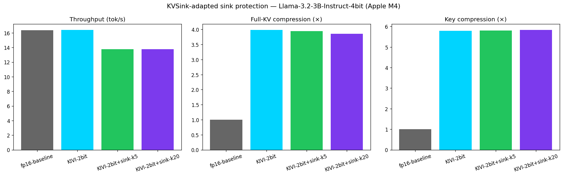
The three panels are, left to right:

• Throughput (tok/s) — generation speed for each config. In this run, enabling sink protection (k=5 or k=20) cost noticeably more than plain KIVI-2bit (13.8 vs 16.4 tok/s); increasing k further from 5 to 20 made no additional difference.
• Full-KV compression (×) — the realistic end-to-end compression ratio, including the fp16 cost of protected sink tokens. This is the panel that actually shows the protection-cost curve described in the script's docstring: it decreases as k grows.
• Key compression (×) — key-cache-only compression. Stays close to flat across all three KIVI/KVSink configs in this run — see the note above on why this isn't the number to use for judging the protection tradeoff.

Try it yourself

--model, --max-tokens, --group-size, and --residual-length all work the same way as in the KIVI example above. Unlike VecInfer and KIVI, this script has no --output-dir flag — output always lands in figures/kivi_sink/<model-stem>/:

PYTHONPATH=. python benchmark_scripts/benchmark_sink.py \
    --model mlx-community/Llama-3.2-3B-Instruct-4bit \
    --max-tokens 256 \
    --group-size 64 \
    --residual-length 64

Interpreting results

Compression ratio

compression_ratio = fp16_equivalent_mb / peak_compressed_mb. Higher is better — a ratio of 8× means the compressed cache uses 8× less memory than fp16.

Cosine similarity

The average cosine similarity between original and quantized keys. A value above 0.95 indicates high fidelity. Below 0.90 may cause noticeable generation quality degradation on some tasks.

Tokens per second

End-to-end throughput including quantization overhead. With Metal kernels, VeloxQuant-MLX typically achieves throughput within 2–5% of fp16 baseline at 2-bit compression.

Reproducing paper numbers

benchmark_scripts/run_outlier_ratequant.py reproduces the Outlier-Token + RateQuant comparison (fp16 baseline vs. RVQ 1-bit vs. RVQ 1-bit + Outlier-Token vs. RVQ + RateQuant per-layer allocation) across 8 models. Per its own module docstring:

# Full 8-model × 4-config sweep — one fresh subprocess per (model, config)
python3 benchmark_scripts/run_outlier_ratequant.py

# Restrict to specific models (comma-separated model keys, not full HF ids)
python3 benchmark_scripts/run_outlier_ratequant.py --models mistral7b,phi4

# Restrict to specific configs
python3 benchmark_scripts/run_outlier_ratequant.py --configs fp16,rvq1o

# Re-run even if cached results exist
python3 benchmark_scripts/run_outlier_ratequant.py --force

# Change the RateQuant per-layer average bit target (default 1.5)
python3 benchmark_scripts/run_outlier_ratequant.py --ratequant-target 1.5

Not run for this guide — verified against source, not executed

This is a genuinely large sweep (8 models × 4 configs, one subprocess each), so it wasn't run to produce this doc — unlike the VecInfer/KIVI/KVSink worked examples above, which were. The flags above are copied from the script's own docstring and its real argparse definition, not guessed. If you run it yourself, results land under figures/outlier_token_ratequant/<model>/, one JSON per (model, config) cached in .bench_tmp/ so re-runs skip already-completed configs unless you pass --force.

Calibration artifacts

Methods that need pre-trained codebooks or smoothing factors (VecInfer, SpectralQuant) self-calibrate on first use and cache the result under ~/.cache/veloxquant/<method>/<model-id>/ — see the VecInfer worked example above. There is no separate python -m veloxquant_mlx precompute step required before running these scripts.

See also

• Observers guide
• Mixed-precision guide
• Core abstractions API